Linear Programming
(Key Points)
① Linear Programming Problems – Problems which concern with finding the minimum or maximum value of a linear function Z (called objective function) of several variables (say x and y), subject to certain conditions that the variables are non-negative and satisfy a set of linear inequalities (called linear constraints) are known as linear programming problems.
② Objective function – A linear function z = ax + by, where a and b are constants, which has to be maximised or minimised according to a set of given conditions, is called a linear objective function.
③ Decision Variables – In the objective function z = ax + by, the variables x, y are said to be decision variables.
④ Constraints – The restrictions in the form of inequalities on the variables of a linear programming problem are called constraints. The condition x ≥ 0, y ≥ 0 are known as non – negative restrictions.
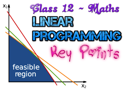
⑤ Feasible Region – The common region determined by all the constraints including non–negative constraints x,y ≥ 0 of linear programming problem is known as feasible region (or solution region) If we had c the region according to the given constraints, then the shaded areas are the feasible region which is the common area of the regions drawn under the given constraints.
⑥ Feasible Solution – Each point within and on the boundary of the feasible region represents the feasible solution of constraints. In the feasible region, there are infinitely many points which satisfy the given condition.
⑦ Optimal Solution – Any point in the feasible region that gives the optimal value (maximum or minimum) of the objective function is called an optimal solution.
⑧ Theorem 1 – Let R be the feasible region (convex polygon) for a linear programming problem and let Z = ax + by be the objective function. When Z has an optimal value (maximum or minimum), where the variables x and y are subject to constraints described by linear inequalities, the optimal value must occur at a corner point of the feasible region.
⑨ Theorem 2 – Let R be the feasible region for a linear programming problem, and let
Z = ax + by be the objective function. If R is bounded them the objective function Z has both maximum and minimum value on R and each of these occurs at a corner point of R.
⑩ Different Types of Linear Programming Problem –
(i) Manufacturing Problems – In such problem, we determine the number of units of different products which should to produced and sold by a firm when each product requires a fixed manpower required, machines hours, labour hour per unit product needed were house space per unit of the output etc., in order to make maximise profit.
(ii) Diet Problem – We determine the number of different types of constituents or nutrients which should be included in a diet so as to minimise the cost of the desired diet such that it contains a certain minimum amount of each constituent/nutrients.
(iii) Transportation Problems – In these problems, we determine a transportation schedule in order to find the cheapest way of transporting a product from plants/factories situated at different locations to different markets.
⑪ Formulation of LPP – Formulation of LPP means converting verbal description of the given problem into mathematical form in terms of objective function, constraints and non-negative restriction:
(i) Identification of the decision variables whose value is to be determined.
(ii) Formation of an objective function as a linear function of the decision variables.
(iii) Identification of the set of constraints or restrictions. Express them as linear inequation with an appropriate sign of equality or inequality.
(iv) Mention the non-negative restriction for the decision variables.
⑫ Steps to solve The LPP –
(i) First of all, formulate the given problem in terms of mathematical constraints and an objective function.
(ii) The constraints would be inequations which shall be plotted and relevant area shall be shaded.
(iii) The corner points of the common shaded area shall be identified and the coordinates corresponding to these points shall be substituted in the objective function.
(iv) The coordinates of one corner point which maximize or minimize the objective function shall be the optimal solution of the given problem. If feasible region is unbounded, then a maximum or a minimum value of the objective function may not exist. However, if it exists, it must occur at a corner point of the feasible region.

No comments:
Post a Comment
We love to hear your thoughts about this post!
Note: only a member of this blog may post a comment.